It does all sound a bit far fetched. Admittedly. But there is a theory or hypothesis for almost every doubt expressed on the subject. In fact, it is often surprising how simple some of the explanations are.
We could state simply that the better a cable is electrically, the better it will sound. However, the exact analogue of this hypothesis as regards amplifiers (that improved THD figures automatically implies improved sound) has been well debunked, so we should be rash to claim that. The point is, both for amplifiers and cables, that the ear functions in such a strange manner (as far as anyone can tell, which isn’t all that far) that “better is not always an obvious direction. In fact, it can be argued very convincingly on philosophical grounds that “better “must always be defined empirically, i.e. by ear, subjectively.
From the point of view of audio design, this is highly unsatisfactory. What is needed in design is a well defined set of design criteria, and subjective judgement is not by any means the best way to derive such. However, one must do the best one can, by correlation between many observations of many phenomena under many circumstances, by many observers. Science ends to come down to this. It’s all very confusing really, especially if one is accustomed to believe in the objectivity of knowledge.
So when we do say the Isolda cable has better electrical properties than other cables, there are two important factors to bear in mind The first is that for a component to be “perfect”, optimum electrical characteristics are a sine qua non. The second is that the cable design arose by application of theoretical principles to a practical situation, with evaluation carried out, ultimately, subjectively.
It is the business of impedance matching in audio cables that raises the most eyebrows. Impedance matching is not normally considered an issue at frequencies where the cable length is less than about a quarter of the signal wavelength. However, cable theory does not in fact predict any variation in wave behaviour with cable length or frequency, as regards reflection from a mistermination. Signal reflection still occurs, but its effects at low frequencies in short cables are over in such a short time, as a proportion of frequency, that they are generally negligible.
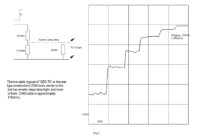
The attached graphs show what happens in various cases when very fast risetime pulses are applied to a length of cable, terminated correctly or otherwise. Basically, the output signal from the cable rises in a staircase fashion, where the width of each step is equal to the transit time along the cable twice (end to end and back), and the height of each step is dependent on the degree of mistermination – gross mistermination gives smaller steps, hence more of them, hence a slower rate of rise. Rate of rise is also slowed by high loss dielectric material.
Bearing this in mind, the ideal cable for any AC application is one which is impedance matched to at least one end and which has very low losses in the dielectric. To see how relevant this was to audio cable, we simply made up some cables complying with this script and tried them out. Unfortunately, the results were sufficiently marked to give us significant pause for thought about how on Earth the ear/brain manages to pick up such apparently subtle effects so clearly. Even more surprising was the effect of reducing series resistance in the cable from low to even lower. We have yet to think of a convincing way of demonstrating the effect of this using test instruments.
As mentioned in the Technical Note on Isolda cable, the most intriguing characteristic of the ear is its extremely refined pitch discrimination ability. The author of this note has measured his own skill at this better than 0.1% frequency shift at 10kHz, and can also tune a concert “A” (440Hz) to about 0.2% absolute. The latter is a less common ability, but the former does not appear to be exceptional. If, as has been suggested, the ear times cycles of a waveform, this could imply that its resolution is less than 100ns. However it does it, this characteristic bears some thinking about.
It has been pointed out that it is not possible to match the impedance of a loudspeaker exactly in a cable, as it varies over quite a wide range. This is true; however, it seems reasonable that one should do the best possible, which means in practice taking an average impedance, in most cases the quoted nominal impedance of the loudspeaker. This minimises the standing wave ratio in the cable. Since standing wave effects are more important at higher frequencies, it is arguably not vital to allow for low frequency aberrations in impedance characteristic, and many loudspeakers have only relatively minor impedance variations above about 4kHz.
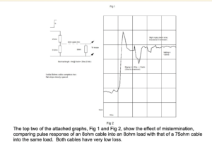
The top two of the attached graphs, Fig 1 and Fig 2, show the effect of mistermination, comparing pulse response of an 8ohm cable into an 8ohm load with that of a 75ohm cable into the same load. Both cables have very low loss.
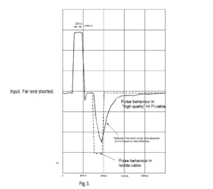
The third graph, Fig 3. shows the effect of poor quality dielectric material: the negative going pulse should be an exact mirror image of the positive going one.
The recent upsurge of interest in audio cables has produced a staggering variety of loudspeaker cables in assorted forms. These cables vary from the simple (house wiring TE) to the complex (MIT shotgun) and from one extreme of bulk (Van Den Hul SCS 2) to the other (DNM). About the only thing these cables have in common is that they have been designed almost exclusively on the basis of an incomplete analysis of the factors affecting “cable sound”
The chief factor and the one most frequently overlooked is the hearing mechanism. The old, “safe” assumptions about human hearing (“the ear has a response from 20Hz to 15 or 20kHZ and is not sensitive to phase, amplitude variations of less than 1db, frequency response nonlinearities of less than 2dB or distortion of less than 0.3%THD”)
Give a drastically incomplete, indeed inaccurate picture; any analogy would be to assert that the Earth is spherical, ignoring completely the equatorial bulge and surface geography. A more nearly complete description assigns to the ear (and internal sound detection mechanisms} a frequency response (highly nonlinear} from 5Hz to 45kHz, a phase sensitivity of perhaps under a microsecond, a rise time of 11us, a sensitivity to amplitude variations of only 0.2dB and frequency shifts of less than 0.05% and a sensitivity to certain forms of linear and nonlinear distortion of 0.01%.
Given these parameters, audio design is seen to be a much less straightforward matter than is frequently assumed. Laboratory instruments regularly achieve better accuracy than is demanded of audio systems, or better frequency response, or better static (linear) distortion, but it is well worth noting that few if any instruments require all of these spefications simultaneously.
The second neglected factor in consideration of audio cables is the interaction of the cable with the transmitting and receiving circuits at either end of it. It is relatively trivial to measure the loss along a piece of cable by differential methods (but see note 3 below), but this does not take into account the behaviour of the driving amplifier when loaded with the cable. (An extreme case is the oscillatory behaviour of certain power amplifiers when connected to a loudspeaker via cable of low inductance- in this case; the amplifier requires the cable inductance to act as part of the Zobel network at its output which maintains stability.) Because of the response of amplifiers, particularly high feedback amplifiers, to very high frequencies, it is necessary to consider cable interaction to frequencies well above the audio band (note 4).
Classical transmission line theory predicts that a transmission line (cable or waveguide) has an associated characteristic impedance, Z, defined for a lossless line as
2 L
Z = C,
where L and C are inductance and capacitance per unit length of line.
When a transmitting or receiving circuit with an output or input impedance equal to Z is connected to such a line there is a complete transfer of power to and from the line with no reflection. If a circuit of impedance not equal to Z is connected, there will be some reflection at the end of the cable. This is true for any frequency, “from DC to daylight”.
“Impedance matching” is employed for example in radio antenna circuits, where a 75ohm aerial feeds a 75ohm input via 75ohm cable.
It is normally assumed that impedance matching is only an issue at frequencies where wavelengths are comparable to the length of cable, since only at frequencies around or above this will standing waves be set up, resulting in drastic power loss and even transmitter damage. However, the wave reflections still occur at lower frequencies, and in the case of a line misterminated at both ends multiple reflections will travel up and down the cable for a long time, depending on the degree of mismatch and the cable loss.
The majority of loudspeaker cables consist of two conductors side by side, insulated with either PVC or PTFE. This form of construction typically gives a characteristic impedance of around 80ohm, which is a poor match to the average loudspeaker impedance of 8ohm and a very poor match to the average amplifier output impedance of around 0.2ohm. Hence reflections can be expected, leading to audible problems. Such widely spaced cables are also susceptible to radio frequency interference and are noticeably sensitive to their surroundings, as the electromagnetic field associated with the signal passing through them is not confined in space.
By contrast, Townshend “Isolda” Impedance Matched cable has a characteristic impedance close to 8ohm for optimum loudspeaker matching and minimum reflections in the audio band. The cable is also comprised of two flat strips, a construction which confines the signal’s EM field within the cable and minimises the effect of surrounding objects and interfering fields.
Additionally, the DC resistance of the cable is low; this is another basic factor affecting cable performance, as can be seen from the very simplest analysis. The low DC resistance and minimal, very high performance dielectric material, ensure that the cable impedance is constant, and losses are low, up to several hundred megahertz.
The Townshend “Isolda” cable satisfies the basic criteria of low loss lumped parameters and matched characteristic impedance. It has very low DC resistance and low loss at high frequencies, a consideration which tends to result in somewhat improved subjective performance in audio cables for reasons which are not immediately obvious (since “high frequencies” means around the GHz region).
Subjectively, the gains in using these cables are surprisingly marked. Compared with other cables, detail and bass performance are much improved. This gives an interesting insight into psychoacoustic phenomena, as the measured performance of different cables tends to be very similar at low frequencies, differences only becoming apparent at relatively high frequencies.
Note 1 there has long been confusion in the hi-fi world about “high capacitance cable”. Townshend cables have a very high capacitance by most standards, 600pF/m. However, the point of impedance matching is that, with an 8ohm load on the end of an 8ohm cable, the amplifier sees only 8ohms (resistive), with no series inductance or shunt capacitance. With high impedance cables, the load is seen in series with some or all of the cable inductance. With cables of lower than 8ohm impedance, the load is seen in parallel with more or less of the cable capacitance. Of course, this only applies to a theoretical 8ohm load, unrepresentative of most loudspeakers, but the deviations are relatively small and the approximation is generally valid. In the extreme case where the loudspeaker impedance tends to infinity, an amplifier might see as much as 6000pF of cable capacitance with 10m of cable. If the amplifier has a high output impedance of 1ohm, the effective time constant is 6ns, equivalent to a -3dB point of 25MHz.
Note 2 Strictly speaking, the equation given above for Z is only accurate when both L and C are loss-free (no series resistance with L or dielectric loss with C). This is true for C as the loss factor (D) of open circuit capacitance of these cables is less than 0.1% at audio frequencies. However, the quality factor (Q) of the short circuit inductance is less than one at frequencies below 3kHz. This prompts two observations. First, a cable with a Q of 100 at 1kHz (say) would have to use 7500sq.mm in both conductors, and would have thickness of 20cm and width of 38cm. Second, measurement at audio frequencies shows that the cable does still behave substantially as a constant impedance cable – load it with 8ohm and measure its input impedance, and the result is purely resistive. Load it with an incorrect impedance, and the load resistor appears in series or parallel with some of the cable inductance or capacitance, depending on the precise resistor value.
Note (3); it is interesting that the “time of flight” of a signal down a typical audio cable should be easily detectable at audio frequencies by differential methods. The speed of light in a typical cable is 200,000,000 m/s; so for a 5m cable the time of flight is 25ns. Thus if a 10kHz input is applied to such a cable at one end, with wave function
V(in) = sin(20,000pi.t)
The output at the other end will be
-8
V(out) = sin20,000pi.(t+2.5×10 ).
Using sin(a+b) = sina.cosb + cosa.sinb, V(in) – V(0ut) is seen to be
-4
V(diff) = 5×10 pi.cos(20,000pi.t), i.e. there should be a difference waveform 90 degrees out of phase with the input, with amplitude approximately 0.0016.V(in) – about 56dB down.
This prediction was verified in practice, implying that differential testing of cables and amplifiers is perhaps not as simple as it may seem. This differential signal is of course not an error signal.
A typical propagation delay in a sold state amplifier is about 150ns, which in a differential test should give a signal at -40dB at 10kHz, -34dB at 20kHz, and -60dB at 1kHz. A valve amplifier on test gave a time delay of 700ns, with associated differential signal of -47dB at 1kHz, -27dB at 10kHz and -21dB (9%) at 20kHz.
Note (4) bearing in mind that in the case of a typical amplifier with feedback from output to input the output impedance is subject to the same “time delay” as a signal passing from input to output (although somewhat counterintuitive, this model is strictly speaking correct), consideration of the effect of cable reflections on a circuit becomes extremely complex.
Note (5); in a very simple experiment, we established that the ear can easily detect a frequency shift of 0.1.% at 10kHz, (This is the best resolution our signal generator would allow.) If one assumes that the ear discriminates frequencies by measuring time intervals between successive zeros or maxima of a waveform, as is suggested by some psychoacoustic research, then it can apparently differentiate between the 100us per cycle of 10kHz and the 99.9us per cycle of 10.01kHz. This in turn implies that the effective resolution of the ear is better than 100ns. If so, the reasons for audible differences between cables are entirely obvious (as, incidentally, are some of the reasons for the inferiority of 44kHz digital recording). The subjective quality of the effects is however still mysterious.